More preliminary topics

Section 1.5 More preliminary topics

Subsection 1.5.1 A useful tool: commutative diagrams

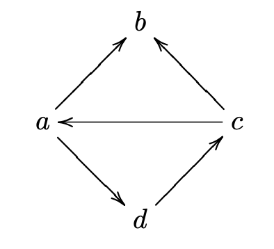
A directed graph (or digraph ) is a set \(V\) of vertices and a set \(E\subset V\times V\) of directed edges. We draw pictures of digraphs by drawing an arrow pointing from a vertex \(v\) to a vertex \(w\) whenever \((v,w)\in E\text{.}\) See Figure 1.5.1.

A path in a directed graph is a sequence of vertices \(v_0,v_1,\ldots,v_{n}\) such that \((v_{i-1},v_i)\in E\) for \(1\leq i\leq n\text{.}\) The vertex \(v_0\) is called the initial vertex and \(v_n\) is called the final vertex of the path \(v_0,v_1,\ldots,v_{n}\text{.}\)

Figure 1.5.1. Example of a directed graph with vertex set \(V=\{a,b,c,d\}\) and edge set \(E=\{(a,b),(c,b),(c,a),(a,d),(d,c)\text{.}\) The vertex sequences \(c,b\) and \(c,a,b\) are both paths from \(c\) to \(b\text{.}\)

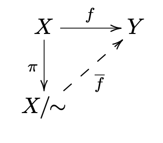
A commutative diagram is a directed graph with two properties.

Vertices are labeled by sets and directed edges are labeled by functions between those sets. That is, the directed edge \(f=(X,Y)\) denotes a function \(f\colon X\to Y\text{.}\)
Whenever there are two paths from an initial vertex \(X\) to a final vertex \(Y\text{,}\) the composition of functions along one path is equal to the composition of functions along the other path. That is, if \(X_0,X_1,\ldots,X_n\) is a path with edges \(f_i\colon X_{i-1}\to X_{i}\) for \(1\leq i\leq n\) and \(X_0=Y_0,Y_1,Y_2,\ldots,Y_m=X_n\) is a path with edges \(g_i\colon Y_{i-1}\to Y_{i}\) for \(1\leq i\leq m\text{,}\) then
\begin{equation*} f_n\circ f_{n-1}\circ\cdots\circ f_1=g_m\circ g_{m-1}\circ\cdots\circ g_1. \end{equation*}

Figure 1.5.2 shows a commutative diagram that illustrates the definition of conjugate transformations. Figure 1.5.3 shows a commutative diagram that goes with Fact 1.4.4.

Figure 1.5.2. A commutative diagram illustrating the definition of conjugate transformations \(f,g\) given in Exercise Group 1.3.4.3–6.

Figure 1.5.3. A commutative diagram showing the relationship \(\overline{f}\circ \pi = f\) in Fact 1.4.4.

Exercises 1.5.2 Exercises

1.

Let \(r\) be a pure, unit quaternion. Use (1.2.13) to show that the map \(\R^3_\Quat \to \R^3_\Quat\) given by \(u\to rur\) is the reflection across the plane normal to \(r\text{.}\) That is, show that \(rur=u-2(u\cdot r)r\text{.}\) See Figure 1.5.4.

Figure 1.5.4. The reflection of \(u\in \R^3_\Quat\) across the plane normal to \(r\in \R^3_\Quat\text{.}\)

2. Commutative diagram examples.

Draw a commutative diagram that illustrates the results of Exercise 1.3.4.5.
The distributive law for \(\Z_n\) says that
\begin{equation*} [x]\left([y]+[z]\right) = [x][y] + [x][z] \end{equation*}
for all \([x],[y],[z]\in \Z_n\text{.}\) Label the maps in the commutative diagram below to express the distributive law.

Figure 1.5.5.

Prev Top Next