Before the discovery of hyperbolic geometry, it was believed that Euclidean geometry was the only possible geometry of the plane. In fact, hyperbolic geometry arose as a byproduct of efforts to prove that there was no alternative to Euclidean geometry. In this section, we present a Kleinian version of hyperbolic geometry.
Definition3.3.1.
Let \(\D=\{z\colon |z|\lt
1\}\) denote the open unit disk in the complex plane. The hyperbolic group, denoted \(\H\), is the subgroup of the Möbius group \(\M\) of transformations that map \(\D\) onto itself. The pair \((\D,\H)\) is the (Poincaré) disk model of hyperbolic geometry.
Comments on terminology: Beware of the two different meanings of the adjective "hyperbolic". To say that a Möbius transformation is hyperbolic means that it is conjugate to a homothety (see Subsection 3.2.6). That is not the same thing as an element of the group of hyperbolic transformations.
Subsection3.3.1The hyperbolic transformation group
Our first task is to characterize transformations in the group \(\H\text{.}\) We begin with an observation about Möbius transformations that map one "side" of a cline to itself. This is pertinent because the disk \(\D\) is the "inside" of the cline which is the unit circle. It will be useful to start with a general case.
Any cline \(C\) divides the extended plane into two regions. If \(C\) is a Euclidean circle, we might called these regions the "inside" and the "outside" of \(C\text{.}\) If \(C\) is a Euclidean straight line, we simply have one side and the other of \(C\text{.}\)
Proposition3.3.2.Möbius transformations that map one side of a cline to itself.
Let \(C\) be a cline, and let \(D,E\) be the two disjoint regions of \(\extC \setminus C\text{.}\) Let \(T\) be a Möbius transformation that maps \(D\) onto itself. Then \(T\) also maps \(E\) onto itself, and \(T\) maps \(C\) onto itself.
Proof.
Sketch: Suppose that \(T\) maps \(D\) onto itself. The "other side" of \(C\) is the set of points that are symmetric, with respect to \(C\text{,}\) to the points in \(D\text{.}\) By Proposition 3.2.26, \(T\) maps symmetric points to symmetric points, so \(T\) maps \(E\) into itself. It is easy to check that, in fact, \(T\) maps \(E\)onto itself. By elimination, it must be that \(T\) maps \(C\) onto itself.
If \(T\in
\H\text{,}\) then \(T\) maps the unit circle onto itself.
Given \(T\in \H\text{,}\) let \(z_0\in\D\) be the point that \(T\) maps to \(0\text{.}\) It must be that \(T\) maps the symmetric point \(1/z_0^\ast\) to \(\infty\text{.}\) Let \(z_1\) be the point that \(T\) maps to \(1\text{.}\) Then \(T\) has the form (see (3.2.3))
A straightforward derivation shows that \(|\alpha|=1\text{,}\) so that we have (3.3.1) below. Another computation establishes an alternative formula (3.3.2) for \(T\in \H\text{.}\) See Exercise 3.3.6.1.
Proposition3.3.5.
A Möbius transformation \(T\) is in \(\H\) if an only if \(T\) can be written in the form
for some \(a,b\in \C\) such that \(|a|^2-|b|^2=1\text{.}\)
Subsection3.3.2Classification of clines in hyperbolic geometry
The clines of Möbius geometry are classified into several types in hyperbolic geometry, as summarized in Table 3.3.6.
Table3.3.6.Clines in hyperbolic geometry
hyperbolic curve type
cline type
hyperbolic straight line
a cline that intersects the unit circle at right angles
hyperbolic circle
a circle completely contained in \(\D\)
horocycle
a circle with all but one point in \(\D\text{,}\) tangent to the unit circle
hypercycle
a cline that intersects the unit circle at a non-right angle
Checkpoint3.3.7.
Show that each of the four categories of clines in Table 3.3.6 is preserved by transformations in the hyperbolic group. That is, show that any transformation in the hyperbolic group takes hyperbolic straight lines to hyperbolic straight lines, takes hyperbolic circles to hyperbolic circles, takes horocycles to horocycles, and takes hypercycles to hypercycles.
Checkpoint3.3.8.
Show that a hyperbolic straight line that contains 0 must be a diameter of the unit circle.
Hint.
Prove the contrapositive: assume \(C\) is a hyperbolic straight line that is also a Euclidean circle, and intersects the unit circle orthogonally at \(p\text{.}\) Give an argument why \(C\) can not contain 0.
Checkpoint3.3.9.
Show that all hyperbolic straight lines are congruent.
Hint.
Start by showing that any hyperbolic straight line is congruent to \(\extR\text{.}\)
Subsection3.3.3Normal forms for the hyperbolic group
In this subsection, we follow the development of normal forms for general Möbius transformations given in Subsection 3.2.6 to derive normal forms and graphical interpretations for transformations in the hyperbolic group. We begin with an observation about fixed points of a Möbius transformation that maps a cline to itself.
Lemma3.3.10.
Let \(T\in \M\) and let \(C\) be a cline. If \(Tz=z\text{,}\) then \(T(z^{\ast C})=z^{\ast C}\text{.}\)
Now let \(T\) be a non-identity element of \(\H\text{.}\) The fact that \(T\) maps the unit circle to itself implies that there are exactly three possible cases for fixed points of \(T\text{.}\)
There is a pair of fixed points \(p,q\) with \(|p|\lt 1\text{,}\)\(|q|\gt 1\text{,}\) and \(q=\frac{1}{p^\ast}\text{,}\) that is, \(p,q\) are a pair of symmetric points (with respect to the unit circle) that do not lie on the unit circle.
There is a pair of fixed points that lie on the unit circle.
There is a single fixed point that lies on the unit circle.
Checkpoint3.3.11.
Give an argument to justify the three cases above.
Figure3.3.12.Three types of hyperbolic transformations
For cases 1 and 2 above, the map \(T\) acting on the \(z\)-plane is conjugate to the map \(U=S\circ T\circ
S^{-1}\) acting on the \(w\)-plane by \(Uw=\lambda w\text{,}\) for some nonzero \(\lambda\in\C\text{,}\) via the map \(w=Sz=\frac{z-p}{z-q}\text{.}\) In case 1, the map \(S\) takes the unit circle to some polar circle, say \(C\text{,}\) so \(U\) must map \(C\) to itself. It follows that \(|\lambda|=1\text{,}\) so the Möbius normal form type for \(T\) is elliptic. The action of \(T\) is a rotation about Steiner circles of the second kind (hyperbolic circles) with respect to the fixed points \(p,q\text{.}\) A transformation \(T\in \H\) of this type is called a hyperbolic rotation. See Figure 3.3.12.
For case 2, the map \(w=Sz=\frac{z-p}{z-q}\) takes the unit circle to a straight line, say \(L\text{,}\) through the origin, so \(U=S\circ T\circ S^{-1}\) must map \(L\) to itself. It follows that \(\lambda\) is real. Since \(S\) maps \(\D\) to one of the two half planes on either side of \(L\text{,}\) the map \(U\) must take this half plane to itself. If follows that \(\lambda\) must be a positive real number, so the Möbius normal form type for \(T\) is hyperbolic. The action of \(T\) is a flow about Steiner circles of the first kind (hypercycles and one hyperbolic straight line) with respect to the fixed points \(p,q\text{.}\) A transformation \(T\in \H\) of this type is called a hyperbolic translation. See Figure 3.3.12.
For case 3, the conjugating map \(w=Sz=\frac{1}{z-p}\) takes \(T\) to \(U=S\circ T\circ S^{-1}\) of the form \(Uw=w+\beta\) for some \(\beta\neq 0\text{.}\) The Möbius normal form type for \(T\) is parabolic. The action of \(T\) is a flow along degenerate Steiner circles (horocycles) tangent to the unit circle at \(p\text{.}\) A transformation \(T\in \H\) of this type is called a parallel displacement. See Figure 3.3.12.
This completes the list of transformation types for the hyperbolic group. See Table 3.3.13 for a summary.
Table3.3.13.Normal forms for the hyperbolic group
hyperbolic transformation type
Möbius normal form
graphical dynamic
hyperbolic rotation
elliptic
flow around hyperbolic circles
parallel displacement
parabolic
flow around horocycles
hyperbolic translation
hyperbolic
flow along hypercycles
(none)
loxodromic
Subsection3.3.4Hyperbolic length and area
Figure3.3.14.Constructing the hyperbolic straight line containing two points \(z_1,z_2\)
Let \(z_1,z_2\) be distinct points in \(\D\text{.}\) Let \(T\in\H\) be the transformation that sends \(z_1\to 0\) and \(z_2\to u\gt 0\text{.}\) Then \(T^{-1}(\R)\) is a hyperbolic straight line that contains \(z_1,z_2\text{.}\) Let \(q_1=T^{-1}(-1)\) and \(q_2=T^{-1}(1)\text{.}\) See Figure 3.3.14.
Checkpoint3.3.15.
Use Proposition 3.3.5 to write a formula for the transformation \(T\) in the previous paragraph.
Solution.
Let \(Sz=\frac{z-z_1}{1-z_1^\ast z}\text{,}\) let \(t=-\arg
(Sz_2)\text{,}\) and let \(Tz=e^{it}Sz\text{,}\) so that we have \(Tz_1=0\) and \(Tz_2=u\gt 0\text{.}\) Because \(T\in \H\text{,}\)\(T\) is determined by the two parameters \(z_1,t\text{.}\)
A simple calculation verifies that \((0,u,1,-1)=\frac{1+u}{1-u}\text{.}\) By invariance of the cross ratio, we have \((z_1,z_2,q_2,q_1)=\frac{1+u}{1-u}\text{.}\) For \(0\leq u\lt
1\text{,}\) we have
where \(q_1,q_2\) are the ideal points on the hyperbolic straight line connecting \(z_1,z_2\) (with each \(q_i\) at the \(z_i\) end of the line) as described above, in the case \(z_1\neq z_2\text{.}\) From the discussion above we have
The following Proposition shows that \(d\) is a metric on hyperbolic space, and justifies referring to \(d(z_1,z_2)\) as the (hyperbolic) distance between the points \(z_1,z_2.\)
Proposition3.3.20.
The function \(d\) given by (3.3.3) defines a metric on \(\D\text{.}\) That is, \(d\) satisfies the following conditions for all \(z_1,z_2,z_3\) in \(\D\text{.}\)
\(d(z_1,z_2)\geq 0\text{,}\) and \(d(z_1,z_2)=0\) if and only if \(z_1=z_2\)
\(\displaystyle d(z_1,z_2)=d(z_2,z_1)\)
\(d(z_1,z_3)\leq d(z_1,z_2)+d(z_2,z_3)\) (the triangle inequality)
Proof.
Property 1 follows immediately from (3.3.4). Property 2 is a simple calculation: just write down the cross ratio expressions for \(d(z_1,z_2)\) and \(d(z_2,z_1)\) and compare. The proof of Property 3 is outlined in exercise Exercise 3.3.6.4.
Now let \(\gamma\) be a curve parameterized by \(t\to z(t)=x(t)
+ iy(t)\text{,}\) where \(x(t),y(t)\) are differentiable real-valued functions of the real parameter \(t\) on an interval \(a\lt t\lt b\text{.}\) Consider a short segment of \(\gamma\text{,}\) say, on an interval \(t_0\leq t\leq
t_1\text{.}\) Let \(z_0=z(t_0)\) and \(z_1=z(t_1)\text{.}\) Then we have \(d(z(t_0),z(t_1))=\ln\left(\frac{1+u}{1-u}\right)\) where \(u=\left|\frac{z_1-z_0}{1-z_0^\ast(z_1)}\right|\text{.}\) The quantity \(|z_1-z_0|\) is well-approximated by \(|z'(t_0)|dt\text{,}\) where \(z'(t)=x'(t)+iy'(t)\) and \(dt=t_1-t_0\text{.}\) Thus, \(u\) is well-approximated by \(\frac{|z'(t_0)|}{1-|z(t_0)|^2}\;dt\text{.}\) The first order Taylor approximation for \(\ln((1+u)/(1-u))\) is \(2u\text{.}\) Putting this all together, we have the following.
Show that the first order Taylor approximation of \(\ln((1+u)/(1-u))\) is \(2u\text{.}\)
Checkpoint3.3.22.
Find the length of the hyperbolic circle parameterized by \(z(t) = \alpha e^{it}\) for \(0\leq t\leq 2\pi\text{,}\) where \(0\lt \alpha\lt 1\) .
We conclude this subsection on hyperbolic length and area with an integral formula for the area of a region \(R\) in \(\D\text{,}\) following the development in [4]. As a function of the two real variables \(r\) and \(\theta\text{,}\) the polar form expression \(z=re^{i\theta}\) gives rise to the two parameterized curves \(r\to z_1(r)=re^{i\theta}\) (where \(\theta\) is constant) and \(\theta \to z_2(\theta) = re^{i\theta}\) (where \(r\) is constant). Using \(z_1'(r) =
e^{i\theta}\) and \(z_2'(\theta)=ire^{i\theta}\text{,}\) the arc length differential \(ds=\frac{2|z'(t)|\;dt}{1-|z(t)|^2}\) for the two curves are the following.
Thus we have \(dA=\frac{4r\;dr\;d\theta}{(1-r^2)^2}\text{,}\) so that the area of a region \(R\) is
\begin{equation}
\text{Area}(R)=\iint_R
dA = \iint_R \frac{4r\;dr\;d\theta}{(1-r^2)^2}.\tag{3.3.7}
\end{equation}
Checkpoint3.3.23.
Find the area of the hyperbolic disk \(\{|z|\leq
\alpha\}\text{,}\) for \(0\lt \alpha\lt 1\text{.}\)
Subsection3.3.5The upper-half plane model
Definition3.3.24.The upper half-plane model of hyperbolic geometry.
Let \(\U=\{z\colon \im(z)\gt
0\}\) denote the half of the complex plane above the real axis, and let \(\HU\) denote the subgroup of the Möbius group \(\M\) of transformations that map \(\U\) onto itself. The pair \((\U,\HU)\) is the upper half-plane model of hyperbolic geometry.
Proposition3.3.25.
A Möbius transformation \(T\) is in \(\HU\) if and only if \(T\) can be written in the form
such that \(a,b,c,d\) are real and \(ad-bc\gt
0\text{.}\)
Hyperbolic straight lines in the upper half-plane model are clines that intersect the real line at right angles. The hyperbolic distance between two points \(z_1,z_2\) in the upper half-plane is
where \(q_1,q_2\) are the points on the (extended) real line at the end of the hyperbolic straight line that contains \(z_1,z_2\text{,}\) with each \(q_i\) on the same "side" as the corresponding \(z_i\text{.}\) The hyperbolic length of a curve \(\gamma\) parameterized by \(t\to
z(t)=x(t)+iy(t)\) on the interval \(a\leq t\leq b\) is
Continue this derivation to show that \(|\alpha|=1\text{.}\)
Prove (3.3.2) by verifying the following. Given \(z_0\in \D\) and \(t\in \R\text{,}\) show that the assignments \(a=\frac{e^{it/2}}{\sqrt{1-|z_0|^2}},
b=\frac{-e^{it/2}z_0}{\sqrt{1-|z_0|^2}}\) satisfy \(|a|^2-|b|^2=1\) and that
Conversely, given \(a,b\in \C\) with \(|a|^2-|b|^2=1\text{,}\) show that the assignments \(t=2\arg a, z_0=-\frac{b}{a}\) satisfy \(z_0\in
\D\text{,}\) and that (3.3.12) holds.
2.Two points determine a line.
Let \(p,q\) be distinct points in \(\D\text{.}\) Show that there is a unique hyperbolic straight line that contains \(p\) and \(q\text{.}\)
Hint.
Start by choosing a transformation that sends \(p\to
0\text{.}\) For uniqueness, use Checkpoint 3.3.8.
3.Dropping a perpendicular from a point to a line.
Let \(L\) be a hyperbolic straight line and let \(p\in\D\) be a point not on \(L\text{.}\) Show that there is a unique hyperbolic straight line \(M\) that contains \(p\) and is orthogonal to \(L\text{.}\)
Hint.
Start by choosing a transformation that sends \(p\to
0\text{.}\) For uniqueness, use Checkpoint 3.3.8.
4.The triangle inequality for the hyperbolic metric.
Show that \(d(a,b)\leq d(a,c)+d(c,b)\) for all \(a,b,c\) in \(\D\) using the outline below.
Show that the triangle inequality holds with strict equality when \(a,b,c\) are collinear and \(c\) is between \(a\) and \(b\text{.}\) Suggestion: This is a straightforward computation using the cross ratio expressions for the values of \(d\text{.}\)
Show that the triangle inequality holds with strict inequality when \(a,b,c\) are collinear and \(c\) is not between \(a\) and \(b\text{.}\)
Let \(p\in \D\) lie on a hyperbolic line \(L\text{,}\) let \(q\in \D\text{,}\) let \(M\) be a line through \(q\) perpendicular to \(L\) (this line \(M\) exists by Exercise 3.3.6.3), and let \(q'\) be the point of intersection of \(L,M\text{.}\) Show that \(d(p,q')\leq d(p,q)\text{.}\) Suggestion: apply \(T\in
\H\) that takes \(p\to 0\) and takes \(L\to
\R\text{.}\) Let \(t=-\arg(Tq)\) if \(\re(Tq)\geq 0\) and let \(t=\pi-\arg(Tq)\) if \(\re(Tq)\lt
0\text{.}\) Let \(r=e^{it}Tq\text{.}\) See Figure 3.3.26.
Given arbitrary \(a,b,c\text{,}\) apply a transformation \(T\) to send \(a\to 0\) and \(b\) to a nonnegative real point. Drop a perpendicular from \(Tc\) to the real line, say, to \(c'\text{.}\) Apply results from the previous steps of this outline.
For the "only if" direction, apply Proposition 3.3.2 to the cline \(\extR\text{,}\) and conclude that \(T\) must send the real line to itself. Set \(z_1,z_2,z_3\) to be the preimages under \(T\) of \(0,1,\infty\text{,}\) and then use (3.2.3). For the "if" direction, suppose \(T\) has the given form. Let \(y\gt 0\) and show that \(\im(T(x+iy))\gt 0\text{.}\)
6.Length integral in the upper half-plane model.
This exercise is to establish (3.3.10). The strategy is to obtain the differential expression
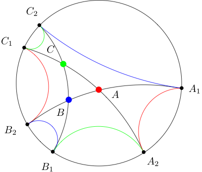
A triangle with one vertex in \(\D\) and two vertices on the unit circle, connected by arcs of circles that are orthogonal to the unit circle, is called a doubly-asymptotic hyperbolic triangle. Examples are \(\triangle AA_1A_2\text{,}\)\(\triangle
BB_1B_2\text{,}\) and \(\triangle CC_1C_2\) in Figure 3.3.27.
Explain why any doubly-asymptotic triangle in the upper half-plane is congruent to the one shown in Figure 3.3.28for some angle \(\alpha\text{.}\)
Now use the integration formula for the upper half-plane model to show that the area of the doubly-asymptotic triangle with angle \(\alpha\) (at the vertex interior to \(\U\)) is \(\pi-\alpha\text{.}\)
Figure3.3.28.Doubly-asymptotic hyperbolic triangle in the upper half-plane with vertices \(1,p,\infty\) with \(p\) on the upper half of the unit circle
9.Area of an asymptotic \(n\)-gon.
A polygon with \(n\geq 3\) vertices on the unit circle, connected by arcs of circles that are orthogonal to the unit circle, is called an asymptotic \(n\)-gon. An example of an asymptotic hexagon is the figure with vertices \(A_1,A_2,B_1,B_2,C_2,C_2\) connected by the colored hyperbolic lines in Figure 3.3.27. Show that the area of an asymptotic \(n\)-gon is \(\pi(n-2)\text{.}\)
Hint.
Partition the asymptotic \(n\)-gon into \(n\) doubly-asymptotic triangles.
10.Area of a hyperbolic triangle.
Let \(\triangle
ABC\) be a hyperbolic triangle. Extend the three sides \(AB\text{,}\)\(BC\text{,}\)\(AC\) to six points on the unit circle. See Figure 3.3.27. Use a partition of the asymptotic hexagon whose vertices are these six points to show that the area of \(\triangle ABC\) is
\begin{equation}
\text{Area}(\triangle
ABC)= \pi-(\angle A +\angle B + \angle C).\tag{3.3.13}
\end{equation}
Hint.
Partition the asymptotic hexagon with vertices \(A_1,A_2,B_1,B_2,C_1,C_2\text{.}\) Start with the six overlapping doubly-asymptotic triangles whose bases are colored arcs and whose vertex in \(\D\) is whichever of \(A,B,C\) matches the color of the base. For example, the two red doubly-asymptotic triangles are \(\triangle AA_1A_2\) and \(\triangle
AC_1B_2\text{.}\)