Early motivation for the development of projective geometry came from artists trying to solve practical problems in perspective drawing and painting. In this section, we present a modern Kleinian version of projective geometry.
Throughout this section, \(\F\) is a field, \(V\) is a vector space over \(\F\text{,}\)\(\Proj(V)=(V\setminus \!\{0\})/\F^\ast\) is the projective space, and \(PGL(V)=GL(V)/\F^\ast\) is the projective transformation group. See Exercise 2.5.3.6 for definitions and details. We will write \([T]\) for the projective transformation that is the equivalence class of the linear transformation \(T\) of \(V\text{.}\)
Subsection3.5.1Projective points, lines, and flats
Points in projective space correspond bijectively to 1-dimensional subspaces of \(V\) via
The set of 1-dimensional subspaces in \(V\text{,}\) denoted \(G(1,V)\text{,}\) is an alternative model space for projective geometry. We will usually denote points in projective space using capital letters, such as \(P\text{,}\)\(Q\text{,}\) etc.
The set of 2-dimensional subspaces in \(V\) is denoted \(G(2,V)\text{.}\) Points in projective space are called collinear if they lie together on a projective line. We will usually denote projective lines using lower case letters, such as \(\ell\text{,}\)\(m\text{,}\) etc.
There is an offset by 1 in the use of the word "dimension" in regards to subsets of \(\Proj(V)\) and the corresponding subspace in \(V\text{.}\) In general, a \(k\)-dimensional flat in \(\Proj(V)\) is a set of the form \(\{[v]\colon v\in G(k+1,V)\}\text{,}\) where \(G(d,V)\) denotes the set of \(d\)-dimensional subspaces of \(V\text{.}\) 1 Flats are also called subspaces in projective space, even though projective space is not a vector space.
Points \(P_1=[v_1],P_2=[v_2],\ldots,P_k=[v_k]\) are said to be in general position if the vectors \(v_1,v_2,\ldots,v_k\) are independent in \(V\text{.}\)
Subsection3.5.2Coordinates
For the remainder of this section, we consider \(V=\F^{n+1}\text{.}\) For readability, we will write \(P=[v]=[x_0,x_1,x_2,\ldots,x_{n}]\) (rather than the more cumbersome \([(x_0,x_1,x_2,\ldots,x_n)]\)) to denote the point in projective space that is the projective equivalence class of the point \(v=(x_0,x_1,x_2,\ldots,x_{n})\) in \(\F^{n+1}\text{.}\) The entries \(x_i\) are called homogeneous coordinates of \(P\text{.}\) If \(x_0\neq 0\text{,}\) then
The numbers \(x_i/x_0\) for \(1\leq i\leq n\) are called inhomogeneous coordinates for \(P\text{.}\) The \(n\) degrees of freedom that are apparent in inhomogeneous coordinates explain why \(\Proj(\F^{n+1})\) is called \(n\)-dimensional. Many texts write \(\F\Proj(n)\text{,}\)\(\F\Proj_n\text{,}\) or simply \(\Proj_n\) when \(\F\) is understood, to denote \(\Proj(\F^{n+1})\text{.}\)
Subsection3.5.3Freedom in projective transformations
In an \(n\)-dimensional vector space, any \(n\) independent vectors can be mapped to any other set of \(n\) independent vectors by a linear transformation. Therefore it seems a little surprising that in \(n\)-dimensional projective space \(\F\Proj_n=\Proj(\F^{n+1})\text{,}\) it is possible to map any set of \(n+2\) points to any other set of \(n+2\) points, provided both sets of points meet sufficient "independence" conditions. This subsection gives the details of this result, called the Fundamental Theorem of Projective Geometry.
Let \(e_1,e_2,\ldots, e_n,e_{n+1}\) denote the standard basis vectors for \(\F^{n+1}\) and let \(e_0=\sum_{i=1}^{n+1}e_i\text{.}\) Let \(v_1,v_2,\ldots,v_{n+1}\) be another basis for \(\F^{n+1}\) and let \(c_1,c_2,\ldots,c_{n+1}\) be nonzero scalars. Let \(T\) be the linear transformation \(T\) of \(\F^{n+1}\) given by \(e_i\to c_iv_i\) for \(1\leq i\leq
n+1\text{.}\) Projectively, \([T]\) sends \([e_i]\to [v_i]\) and \([e_0]\to [\sum_i c_iv_i]\text{.}\)
Now suppose there is another map \([S]\) that agrees with \([T]\) on the \(n+2\) points \([e_0],[e_1],[e_2],\ldots,[e_{n+1}]\text{.}\) Then \([U]:=[S]^{-1}\circ
[T]\) fixes all the points \([e_0],[e_1],[e_2],\ldots,[e_{n+1}]\text{.}\) This means that \(Ue_i=k_ie_i\) for some nonzero scalars \(k_1,k_2,\ldots,k_{n+1}\) and that \(Ue_0=k'e_0\) for some \(k'\neq 0\text{.}\) This implies
so we have \(k'=k_1=k+2=\cdots k_{n+1}\text{.}\) Therefore \([U]\) is the identity transformation, so \([S]=[T]\text{.}\) We have just proved the following existence and uniqueness lemma.
Lemma3.5.1.
Let \(v_1,v_2,\ldots,v_{n+1}\) be an independent set of vectors in \(\F^{n+1}\) and let \(v_0=\sum_{i=1}^{n+1}c_iv_i\) for some nonzero scalars \(c_1,c_2,\ldots,c_{n+1}\text{.}\) There exists a unique projective transformation that maps \([e_i]\to [v_i]\) for \(0\leq i\leq n+1\text{.}\)
Theorem3.5.2.Fundamental Theorem of Projective Geometry.
Let \(P_0,P_1,P_2,\ldots,P_{n+1}\) be a set of \(n+2\) points in \(\Proj(\F^{n+1})\) such that all subsets of size \(n+1\) are in general position. Let \(Q_0,Q_1,Q_2,\ldots,Q_{n+1}\) be another such set. There exists a unique projective transformation that maps \(P_i\to Q_i\text{,}\)\(0\leq i\leq n+1\text{.}\)
Subsection3.5.4The real projective plane
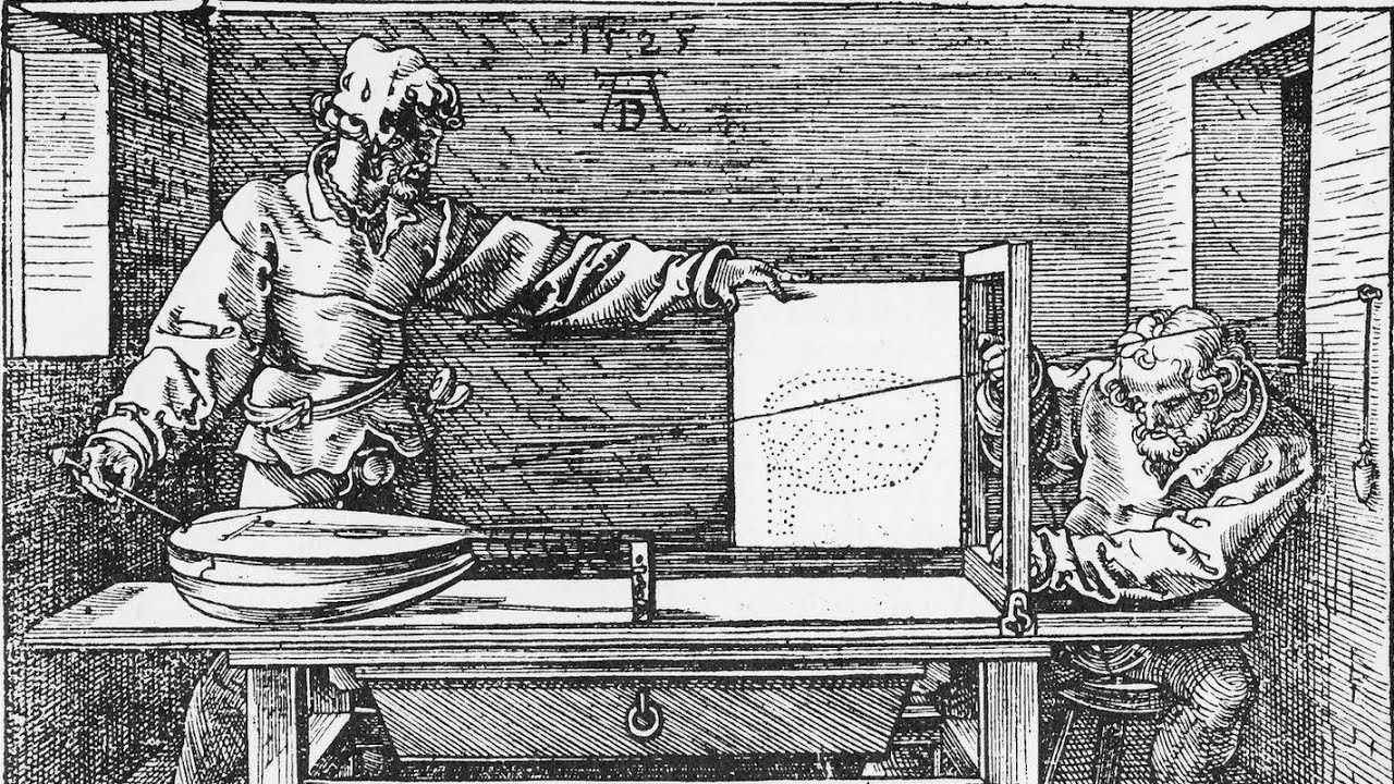
The remainder of this section is devoted to the planar geometry \(\Proj(\R^3)=\R\Proj_2\) called the real projective plane. It is of historical interest because of its early practical use by artists. Lines through the origin in \(\R^3\) model sight lines in the real world as seen from an eye placed at the origin. A plane that does not pass through the origin models the "picture plane" of the artist’s canvas. Figure 3.5.3 shows a woodcut by Albrecht Dürer that illustrates a "perspective machine" gadget used by 16th century artists to put the projective model into practice for image making.
Figure3.5.3.Man drawing a lute, Albrecht Dürer, 1525.
A two dimensional subspace \(\Pi\) in \(\R^3\) is specified by a normal vector \(n=(n_1,n_2,n_3)\) via the equation \(n\cdot v=0\text{,}\) that is, a point \(v=(x,y,z)\) lies on \(\Pi\) with normal vector \(n\) if and only if \(n\cdot
v=n_1x+n_2y+n_3z=0\text{.}\) Any nonzero multiple of \(n\) is also a normal vector for \(\Pi\text{,}\) so the set \(G(2,\R)\) of 2-dimensional subspaces in \(\R^3\) is in one-to-one correspondence \(\R^3/\R^\ast\text{.}\) We will write \(\ell=[n]=[n_1,n_2,n_3]\) to denote the projective line \(\ell\) whose corresponding 2-dimensional subspace in \(\R^3\) has normal vectors proportional to \((n_1,n_2,n_3)\text{.}\) Beware the overloaded notation! Whether the equivalence class \([v]\) of a vector \(v\) in \(\R^3\) denotes a projective point or a projective line has to be specified.
The equation \(n\cdot v=0\) makes sense projectively. This means that if \(n\cdot
v=0\) for vectors \(n,v\text{,}\) then
even though the value of the dot product is not well-defined for projective equivalence classes! Thus we will write \(\ell\cdot P=[n_1,n_2,n_3]\cdot [x,y,z]=0\) for a projective line \(\ell=[n_1,n_2,n_3]\) and a projective point \(P=[x,y,z]\text{,}\) to mean (3.5.1), and we make the following interpretation of the dot product as an incidence relation in \(\R\Proj_2\text{.}\)
Given two independent vectors \(v,w\) in \(\R^3\text{,}\) their cross product \(v\times w\) is a normal vector for the 2-dimensional space spanned by \(v,w\text{.}\) Given two 2-dimensional subspaces \(\Pi,\Sigma\) in \(\R^3\) with normal vectors \(n,m\text{,}\) the cross product \(n\times m\) is a vector that lies along the 1-dimensional subspace \(\Pi\cap\Sigma\text{.}\) The bilinearity of cross product implies that cross product is well-defined on projective classes, i.e., we can write \([u]\times [v]:=[u\times v]\text{.}\) Thus we have the following.
Proposition3.5.4.
Given two points \(P=[u],P'=[u']\) in \(\R\Proj_2\text{,}\) there is a unique projective line \(\overline{PP'}=[u\times u']\) that contains them. Given two lines \(\ell=[n],\ell'=[n']\) in \(\R\Proj_2\text{,}\) there is a unique projective point \([n\times n']\) in their intersection \(\ell\cap \ell'\text{.}\)
Instructor’s solution for Exercise 3.5.5.1 (proof of the Fundamental Theorem of Projective Geometry).
Let \(P_0,P_1,P_2,\ldots,P_{n+1}\) be a set of \(n+2\) points in \(\Proj(\F^{n+1})\) such that all subsets of size \(n+1\) are in general position. Let \(v_0,v_1,v_2,\ldots,v_{n+1}\) be vectors in \(\F^{n+1}\) such that \(P_i=[v_i]\text{.}\) By assumption, the points \(P_1,P_2,\ldots,P_{n+1}\) are in general position, so the vectors \(v_1,v_2,\ldots,v_{n+1}\) are independent and form a basis of \(\F^{n+1}\text{.}\) Let \(c_1,c_2,\ldots,c_{n+1}\) be scalars such that \(v_0=\sum_{i=1}^{n+1}c_iv_i\text{.}\) By Lemma 3.5.1, there is a unique projective transformation \(T\) that maps \([e_i]\to
P_i\text{,}\)\(0\leq i\leq n+1\text{.}\) By the same argument, there is a unique projective transformation \(S\) that maps \([e_i]\to Q_i\text{,}\)\(0\leq i\leq n+1\text{.}\) It follows that the projective transformation \(S\circ T^{-1}\) maps \(P_i\to Q_i\text{,}\)\(0\leq i\leq n+1\text{.}\) For uniqueness, suppose there are two projective maps, say \(U,V\) that map \(P_i\to Q_i\text{,}\)\(0\leq i\leq
n+1\text{.}\) It then follows that \(U\circ T, V\circ T\) both map \([e_i]\to Q_i\text{,}\)\(0\leq i\leq n+1\text{.}\) By the uniqueness statement in Lemma 3.5.1, we have \(U\circ T=V\circ T\text{.}\) Thus we have
Alternatively, we could have stated and proved a separate lemma that says that any projective transformation that fixes \(n+2\) points in \(\Proj(\F^{n+1})\) must be the identity. [The special case of this statement, that we already know, is that a Möbius transformation with three fixed points is the identity.]
2.Coordinate charts and inhomogeneous coordinates.
To facilitate thinking about the interplay between the projective geometry \(\Proj(\F^{n+1})=\F\Proj_n\) and the geometry of \(\F^{n}\) (rather than \(\F^{n+1}\text{!}\)) it is useful to have a careful definition for "taking inhomogeneous coordinates in position \(i\)". Here it is: Let \(U_i\) be the subset of \(\F\Proj_n\) of points whose homogeneous coordinate \(x_i\) is nonzero. Let \(\pi_i\colon U_i\to
\F^n\) be given by
(where the circumflex hat indicates a deleted item from a sequence) is called the \(i\)-th coordinate chart for \(\F\Proj_n\text{.}\) What is the map that results from applying the \(0\)-th coordinate chart \(\C\to \C\Proj_2\) followed by taking homogeneous coordinates in position 1?
Instructor’s solution for Exercise 3.5.5.2.
The map \(\pi_1\circ \text{chart}_0\) is inversion, as follows.
Show that Möbius geometry \((\extC,\M)\) and the projective geometry \((\Proj(\C^2),PGL(2))\) are equivalent via the map \(\mu\colon \Proj(\C^2) \to \extC\) given by
Comment: Observe that \(\mu\) is an extension of \(\pi_1\colon
U_1\to \C\) given by \(\pi_1([x_0,x_1])=\frac{x_0}{x_1}\) (defined in Exercise 3.5.5.2).
Instructor’s solution for Exercise 3.5.5.3.
It is clear that \(\mu\) is a bijection. Let \(T\in
\M\) be given by \(Tz=\frac{az+b}{cz+d}\text{.}\) Let \(M\in
GL(2,C)\) be given by \(M=\twotwo{a}{b}{c}{d}\text{.}\) If \(\beta\neq 0\text{,}\) we have
Thus we have \(\mu\circ T\circ \mu{-1} = [M]\in PGL(2,\C)\) and \(\mu^{-1}\circ [M]\circ \mu = T\in \M\text{.}\)
4.Cross ratio.
The projective space \(\Proj_1=\Proj(\F^2)\) is called the projective line). The map \(\mu\colon \Proj_1\to \extF\text{,}\) given by \(\mu([x_0,x_1])=\frac{x_0}{x_1}\) (defined in Exercise 3.5.5.3, but where \(\F\) may be any field, with \(\extF=\F\cup \{\infty\}\)) takes the points
in \(\Proj_1\) to the points \(1,0,\infty\) in \(\extF\text{,}\) respectively. Let \((\cdot,P_1,P_2,P_3)\) denote the unique projective transformation \([T]\) that takes \(P_1,P_2,P_3\) to \([e_0],[e_2],[e_1]\text{.}\) The cross ratio \((P_0,P_1,P_2,P_3)\) is defined to be \(\mu([T](P_0))\text{.}\)
Show that this definition of cross ratio in projective geometry corresponds to the cross ratio of Möbius geometry for the case \(\F=\C\text{,}\) via the map \(\mu\text{,}\) that is, show that the following holds.
where \(\det(P_iP_j)\) is the determinant of the matrix \(\twotwo{a_i}{a_j}{b_i}{b_j}\text{,}\) where \(P_i=[a_i,b_i]\text{.}\)
Instructor’s solution for Exercise 3.5.5.4.
Let \(S=(\cdot,\mu(P_1),\mu(P_2),\mu(P_3))\text{.}\) By Exercise 3.5.5.3, the map \(\mu^{-1}\circ S\circ \mu\) is a projective transformation, and it is easy to see that \(\mu^{-1}\circ S\circ \mu\) takes \(P_1,P_2,P_3\) to \([e_0], [e_2],[e_1]\text{,}\) so by the Fundamental Theorem of Projective Geometry, we must have \(\mu^{-1}\circ S\circ \mu = [T]\text{.}\) Evaluating both sides of this equation at \(P_0\text{,}\) we have
Let \(u=(u_1,u_2,u_3),v=(v_1,v_2,v_3),w=(w_1,w_2,w_3)\) be vectors in \(\R^3\text{,}\) and let \(M\) be the matrix \(M=\left[\begin{array}{ccc}
u_1 \amp v_1 \amp w_1\\
u_2 \amp v_2 \amp w_2\\
u_3 \amp v_3 \amp w_3\\\end{array}\right]\) Show that \([u],[v],[w]\) are collinear in \(\R\Proj_2\) if and only if \(\det M=0\text{.}\)
Instructor’s solution for Exercise 3.5.5.5.
A line in projective space \(\R\Proj_2\) the set of equivalence classes of all vectors in a 2-dimensional subspace of \(\R^3\text{.}\) The three vectors \(u,v,w\) lie in a 2-dimensional subspace together if and only if the three vectors are linearly dependent. This holds if and only if the determinant of the given \(3\times 3\) matrix is zero.
Figure3.5.5.Pappus’ Theorem
6.
The following is a famous theorem of classical geometry.
Pappus’ Theorem.
Let \(A,B,C\) be three distinct collinear points in \(\R\Proj_2\text{.}\) Let \(A',B',C'\) be another three distinct collinear points on a different line. Let \(P,Q,R\) be the intersection points \(P=BC'\cap B'C\text{,}\)\(Q=AC'\cap
A'C\text{,}\)\(R=AB'\cap A'B\text{.}\) Then points \(P,Q,R\) are collinear. See Figure 3.5.5.
Follow the outline below to prove Pappus’ Theorem under the additional assumption that no three of \(A,A',P,R\) are collinear. Applying the Fundamental Theorem of Projective Geometry, we may assume \(A=[e_1]\text{,}\)\(A'=[e_2]\text{,}\)\(P=[e_3]\text{,}\) and \(R=[e_0]\text{.}\)
Check that \(AR=[0,-1,1]\) and \(A'R=[1,0,-1]\text{.}\)
Explain why it follows that \(B'=[r,1,1]\) and \(B=[1,s,1]\) for some \(r,s\text{.}\)
Explain why \(C=[rs,s,1]\) and \(C'=[r,rs,1]\text{.}\)
Explain why \(Q=[rs,rs,1]\text{.}\)
Observe that \(P,Q,R\) all lie on \([1,-1,0]\text{.}\)
For the second bullet point, use the fact that \(B'=[x,y,z]\) lies on \(AR\) to get \(y=z\text{.}\) For the third bullet point, use known coordinates for \(A,B,B',P\) to get coordinates for lines \(AB,PB'\text{.}\) Then \(C= AB\cap PB'\text{.}\) Use a similar process for \(C'\text{.}\) Four the fourth bullet point, use \(Q=AC'\times A'C\text{.}\)
Instructor’s solution for Exercise 3.5.5.6 (proof of Pappus’ Theorem).
Since \(B'\) lies on \(AR\text{,}\) we have \(B'\cdot
AR=0\text{,}\) so \(B'=[r,x,x]\) for some \(r,x\text{.}\) It must be that \(x\neq 0\text{,}\) for otherwise, we would have \(B'=A\text{.}\) So we can take \(B'\) to be \([r,1,1]\text{.}\) Similar reasoning yields \(B = [1,s,1]\) for some \(s\text{.}\)
Now we have \(C=AB\times PB'=[rs,s,1]\text{.}\) Similar reasoning applies to \(C'\text{,}\) which lies on \(A'B'\) and also on \(BP\) and yields \(C'=[r,rs,1]\text{.}\)
Point \(Q\) lies on \(AC'=[0,-1,rs]\) and also on \(A'C=[1,0,-rs]\text{,}\) so must have the form \(AC'\times A'C=[rs,rs,1]\text{.}\)
We have \(X\cdot [1,-1,0]=0\) for \(X=P,Q,R\text{,}\) so we conclude that \(P,Q,R\) are collinear.
7.Quadrics.
A quadric in \(\Proj(\F^{n+1})\) is a set of points whose homogeneous coordinates satisfy an equation of the form
What are the figures in \(\R^2\) that result from taking inhomogeneous coordinates (see Exercise 3.5.5.2) on \(C\) in positions \(0,1,2\text{?}\)
Instructor’s solution for Exercise 3.5.5.7.
Given a vector \(x=(x_0,x_1,\ldots,x_{n+1})\in\F^{n+1}\text{,}\) let \(c(x)\) denote the expression on the left side of (3.5.4). We have \(c(kx) = k^2c(x)\) for any scalar \(k\text{,}\) so \(c(x)=0\) if and only if \(c(kx)=0\text{.}\)
Taking inhomogeneous coordinates in position 0, let \(u=x_1/x_0,v=x_2/x_0\text{.}\) The points \((1,u,v)\) satisfy \(1+u^2-v^2=0\text{,}\) which is the equation for a hyperbola in the \(u,v\)-plane. Taking inhomogeneous coordinates in position 1 is also a hyperbola. Taking inhomogeneous coordinates in position 2, with \(u=x_0/x_2,v=x_1/x_2\text{,}\) we have \(u^2+v^2-1=0\text{,}\) which is the equation for the unit circle in the \(u,v\)-plane.
The set \(G(d,V)\) is called the Grassmannian of \(d\)-dimensional subspaces of \(V\text{,}\) named in honor of Hermann Grassmann.